Optimizing Geospatial Workloads

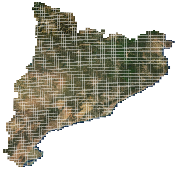
Large area geospatial processing often involves splitting into smaller working tiles to be processed or downloaded independently. As an example, 25cm resolution orthophoto production in Catalonia is divided into 4275 rectangular tiles, as seen in the following image.

Whenever a process can be applied to those tiles independently (ie, not depending on their neighborhood), parallel processing is an easy way to increase the throughput. In such environments, the total workload has to be distributed among a fixed, often limited, number of processing units (be they cores or computers). If the scheduling mechanism requires a predefined batch to be assigned to each core (or if there is no scheduling mechanism at all), and when the processing units are of similar processing power, then the maximum speedup is attained when all batches have an equal amount of tiles.

Furthermore, since the result often has to be mosaicked in order to inspect it, or to aggregate it into a larger final product, it is desireable for the different batches to keep a spatial continuity, ideally conforming axis parallel rectangles, since that is the basic form of georeference for geospatial imagery once projected.

The problem

This is a discrete optimization problem, which can be solved using the regular machinery. Since I have been dusting off my MiniZinc abilities through Coursera’s discrete optimization series, I decided to give it a go.

Tile scheme representation

For convenience, the list of valid tiles can be read from an external .dzn data file.

ntiles = 4275;
Tiles  = [| 253, 055
          | 254, 055
          | 253, 056
          | 254, 056
          | 255, 055
          | 255, 056
          | 256, 056
          | 257, 056
          | 252, 059
          …
          |];

The above basically declares the list of valid tiles as a 2d array with ntiles rows and 2 columns. Then, in our model file (.mzn) the data will be loaded into the Tiles constant array, declared as follows:

int: ntiles;

enum e_tile = { col, row };
array[1..ntiles, e_tile ] of int: Tiles;

Notice the use of a column enum to make access easier.

From the above data, a 2d grid can be built within the bounds of minimum and maximum columns, where the grid value is true if there exists a tile in that position, and false otherwise. This builds a nice representation for modelling the spatial restrictions in the problem.

int: mincol = min([ Tiles[i, ocol] | i in 1..ntiles ]);
int: maxcol = max([ Tiles[i, ocol] | i in 1..ntiles ]);
int: minrow = min([ Tiles[i, orow] | i in 1..ntiles ]);
int: maxrow = max([ Tiles[i, orow] | i in 1..ntiles ]);

array[minrow..maxrow, mincol..maxcol] of int: Grid =
  array2d(minrow..maxrow, mincol..maxcol,
     [ exists(i in 1..ntiles)(Tiles[i, orow] == r /\ Tiles[i, ocol] == c)
       | r in minrow..maxrow, c in mincol..maxcol ]);

Note that all this is computed at compile time, before the actual optimization begins.

Box representation

Boxes are rectangles defined defined by their left, bottom and top bounds:

int: nboxes;
enum e_bbox  = { top, left, bottom, right };
array[1..nboxes, e_bbox] of var int: Boxes;

Grid positions increase like in a matrix (first row top, left column first), and their bounds are constrained within the tile grid limits. Limits are inclusive. These requirements can be expressed as a minizinc constraint:

constraint
  forall(b in 1..nboxes) (
      mincol <= Boxes[b, left] /\ Boxes[b, left]  <= maxcol /\
      minrow <= Boxes[b, top] /\ Boxes[b, top] <= maxcol /\
      Boxes[b, left] <= Boxes[b, right] /\
      Boxes[b, top] <= Boxes[b, bottom]);

Each tile belongs to just one box, so boxes do not overlap.

predicate no_overlap(var int:l1, var int:t1, var int:b1, var int:r1,
                     var int:l2, var int:t2, var int:b2, var int:r2) =
   r1 < l2 \/ l1 > r2 \/ b1 < t2 \/ t1 > b2 \/
   r2 < l1 \/ l2 > r1 \/ b2 < t1 \/ t2 > b1;

constraint 
forall(b1,b2 in 1..nboxes where b1 < b2) (
    no_overlap(
     	Boxes[b1, left], Boxes[b1, top], Boxes[b1, bottom], Boxes[b1, right],
	    Boxes[b2, left], Boxes[b2, top], Boxes[b2, bottom], Boxes[b2, right]));

Assignment

In the end we want an array relating every tile with its box. Since we chose to represent a tile by its row and column, this can be modeled as a 2d array of nboxes. We will reserve a special 0 value for the empty tiles within the grid.

array[minrow..maxrow, mincol..maxcol] of var 0..nboxes: Assignment;

The rules that relate the tile Grid with the Boxes and Assignment vector can be enumerated as follows:

1. Every tile inside the range of a box is assigned to it.
2. Tiles not present are not assigned.
3. Tiles not assigned to a box, but present, are assigned to another box.

constraint
  forall(b in 1..nboxes) (
      forall(r in minrow..maxrow) (
          forall(c in mincol..maxcol) (
            if Grid[r,c] > 0 then
              if contains(Boxes[b, left], Boxes[b, top],
                          Boxes[b, bottom], Boxes[b, right],
                          r, c)Ti
              then
                % 1 - Tiles within the range of a box are assigned to it
                Assignment[r,c] = b
              else
                % 3 - Tiles not assigned to a box are assigned to another
                Assignment[r,c] != b /\ Assignment[r,c] > 0
              endif
            else
              % 2 - Tiles not present are not assigned
              Assignment[r,c] = 0
            endif)));

Objective function

We want to make the resulting rectangles as equal as possible. In order to do so, we have to gather the cardinalities of each box.

array[1..nboxes] of var int: BoxCardinality =
  [ sum(r in minrow..maxrow, c in mincol..maxcol)(Grid[r,c] > 0 /\ Assignment[r,c] == b) | b in 1..nboxes];

This can be done by minimizing the variance, which is the same as minimizing the square L2 norm (dot product of a vector with itself).

var int: variance = sum(b in 1..nboxes)(BoxCardinality[b]*BoxCardinality[b]);
solve minimize variance;

Showing the results

It is useful to dump the result in some format that can be easily parsed by standard command-line tools, since some models have to be further processed. In this case, the lines corresponding to the assignment vector are prefixed with the tag Tiles to make them easy to redirect to another file.

The printing itself can be done with a combination of helper functions and array comprehensions.

function string: show_assignment(int: r, int: c) = "Tile: " ++ show(c) ++ "-" ++ show(r) ++ "," ++ show(Assignment[r,c]) ++ "\n";

output 
  [ show_assignment(r,c) | r in minrow..maxrow, c in mincol..maxcol where Grid[r,c] > 0 ] ++ 
  [ "Variance: ", show(variance), "\n",
    "Box Cardinalities: ",  show(BoxCardinality) , "\n" ];

For powershell users, this could be captured, for example:

$ENV:FLATZINC_CMD = "fzn-gecode"
$Env:PATH += ";D:\Soft\MiniZinc\"
minizinc.exe -I D:\Soft\MiniZinc\share\minizinc\gecode\ .\tall5m.mzn .\tall5m.dzn | ? { $_ -match "Ortho: " } | % { $_ -replace "Ortho: " } | out-file -encoding ascii assign5.csv

Not so fast!

For big grids, the process is too slow (on my hardware, ymmv). A practical way to mitigate that problem is including further “artificial” restrictions that capture some common-sense knowledge. Here we can set that box cardinalities belong to an environment around a perfect one, which would happen when every box has ntiles / nboxes tiles.

We can define a parameter slack, that will represent the radius of the environment, and add the following constraint:

% All boxes have at least one tile assigned to it
float: fill_factor = (ntiles / nboxes);

constraint
   forall(b in 1..nboxes) ( (1.0 - slack)*fill_factor <= BoxCardinality[b] /\ BoxCardinality[b] <= (1.0 + slack)*fill_factor ) ; 

This is common in discrete optimization problems, where a hybrid system can be developed. In this case, we could use some sort of search to optimize for the value of the slack, with different invocations of minizinc.

Results

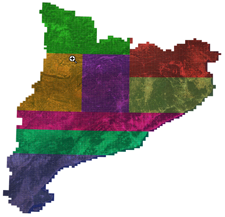
By processing the results of minizinc and joining the results into a QGis project, we can easily map the box assignment. Here is the result for 4 boxes:

For 8 boxes (8 parallel processors), the result would be:

Conclusions

Even when I know the basic theory behind mixed integer and fp solvers (even implemented a simplex-based solver as a practical exercise in the past), I keep having the feeling there is some form of magic at work here.

There are lots of other ways to model this problem. In particular, MiniZinc has special primitives for dealing with sets. Some of the restriction explicitly stated by the model are already available for reuse in the globals library, which would probably more efficient and would lead to terser code. I would like to rewrite the model using these functions and compare their efficiency if I ever have the time.

For now, I got my results!